evolution of how ai makes videos

some of you might remember this hilarious clip of distorted Will Smith trying to enjoy some pasta back in 2022/2023.

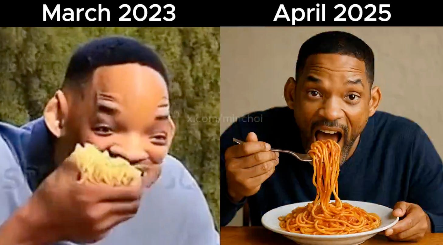
full video comparison here.

ai video generation models have come a very long way from this janky in 2023 to present day 2025.

a lot of mainstream focus has been on LLMs and their performance against popular benchmarks like CoderBench and AIME. these frontier models have definitely improved substantially; i use them every day to write code, write my work emails, and write sorry notes to my girlfriend.

while these models are definitely showing promise in automating my life, a very slept on category of generative ai is the innovation with video models. this could be because the models out there aren’t “100% perfect”, however an overview of recent progress really demonstrates that we are paving a road to truly getting “100% there”.

let’s take a look at the recent evolution of ai video generation models.

background

skip to the bottom line of this section if you don’t care to understand the math.

it is important to get a basic grasp of how denoising diffusion probabilistic models (DDPM) work. DDPM is a generative model that learns to gradually reverse a noise-adding process; in other words, transforming noise into coherent data like an image or video.

training process (forward diffusion process):

$$\begin{align} q(\mathbf{x}_{1:N} \mid \mathbf{x}_0) &= \prod_{n=1}^{N} q(\mathbf{x}_n \mid \mathbf{x}_{n-1}) \\ q(\mathbf{x}_n \mid \mathbf{x}_{n-1}) &= \mathcal{N}\!\left(\mathbf{x}_n \mid \sqrt{1 - \beta_n}\,\mathbf{x}_{n-1}, \, \beta_n \mathbf{I}\right) \end{align}$$

the top formula is simply stating that the forward diffusion process to get from the first diffusion step to the Nth diffusion step can be represented by a first-order Markov chain. this is a mathematical way of saying that to get from x_n-1 to x_n, you only need to know the state of x_n-1 (sorry substack does not support inline math LaTeX).

the bottom formula describes one step of adding noise. it says that the probability of x_n given x_n-1 can be modelled using a gaussian distribution where the mean is equal to the square root of 1 - beta_n times x_n-1, and the covariance is beta_n times I, which is another way of writing the isotropic Gaussian noise.

inference process (reverse denoising process):

$$\begin{align} p_{\theta}(\mathbf{x}_{0:N}) &= p(\mathbf{x}_N) \prod_{n=1}^{N} p_{\theta}(\mathbf{x}_{n-1} \mid \mathbf{x}_n), \\ p_{\theta}(\mathbf{x}_{n-1} \mid \mathbf{x}_n) &= \mathcal{N}\!\left(\mathbf{x}_{n-1} \;\middle|\; M_{\theta}(\mathbf{x}_n, n), \; \gamma \mathbf{I}\right). \end{align}$$

the top formula also states that the denoising process is modelled after a first-order Markov chain.

the only difference with the bottom formula is that the mean function is now learned with hyperparameter theta. so during training, we are trying to learn how to denoise at each step.

bottom line: diffusion models are trained by taking an image, and then iteratively adding noise to it. the model is made to try and predict how much noise was added at a given step. at generation time, it is the reverse, which is starting from noise and then removing the noise that it predicts until you get the end result.

genesis

let’s start back in 2022. at this point in time, diffusion models have done an extremely good job at producing high quality results for image and audio generation.

on April 7, 2022 a study from Google introduced the ‘Video Diffusion Model’ [1]. the main innovation was the Video U-Net (also called 3D U-Net) architecture. this was essentially an extension of the Gaussian diffusion model for images, which used the U-Net architecture.

2D U-Net only used spatial convolutions using a 2D kernel (height x width). the 3D U-Net extends this by factorizing 3D convolutions into standard 2D spatial convolutions and lightweight temporal modules. In addition to these higher dimensional convolutions, they employed both spatial attention layers and temporal attention layers for more coherence for the generated videos.

another important note is the use of factorized space-time attention. this allowed the model to be trained on both images and videos. this is very beneficial due to the plethora of image data available, compared to the scarcity of video data.

on October 5, 2022, Google leveraged this architecture and released the first version of Imagen, one of the first ‘impressive’ text-to-video (T2V) models [2]. Imagen introduced a cascade architecture that is built using Video U-Net (Base model in the diagram), as well as text-conditioning.

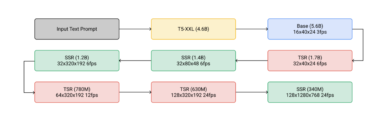
Imagen’s cascade architecture.

around the same time, Meta released their own model called Make-a-Video on September 29, 2022 [3]. Make-a-video is another one of the first large scale T2V models that showed a level of fluidity between frames.

Make-a-video breaks the dependency on text-video pairs for T2V generation, which is key to remove the restriction of generating videos of a narrow domain or requiring large scale paired text-video data.

while Imagen and Make-a-video are similar in terms of a cascade structure, Make-a-video primarily differs by their usage of ‘pseudo 3D layers’ instead of Video U-Net. Imagen designed a factorized 3D U-Net from scratch, while Make-a-video basically retrofitted an existing, pre-trained image diffusion model, and just added the temporal modules by adding a 1D convolution across the frames.

these initial efforts were significant strides forward for video models, but it still suffered from expensive compute and memory, limited video resolution, and inability to maintain object coherence across longer timescales.

beyond pixel diffusion

many of the major models including Imagen and Make-a-video operated directly in pixel space. if you are aware of how LLMs work, you will know that we embed words as tokens and work in what is called the ‘latent space’.

just as LLMs don’t work with raw characters but on compact embeddings diffusion models can also move from pixel space into a compressed latent representation. on April 18, 2023, NVIDIA released a study developing one of the first major Latent Diffusion Models (LDM) [4].

one of the major problems with early T2V pixel-space models is how compute-hungry they were. take for instance a 128-frame 1280x768 resolution RGB video. for this one video, you would need to compute 128 x 1280 x 768 x 3 ≈ 377,487,360 numbers. that works out to roughly 377,487,360 x 4 ≈ 1.51 GB of memory for a single video (assuming float32). scaling this to a batch of 16 videos, this means you need about 24 GB of memory for just the raw inputs. this does not even account for model parameters, etc.

if we instead take that same video, and transform it into latent space, we would do a spatial reduction by 8, and a temporal reduction by 4. So instead of roughly 378M numbers, it would be 128/4 x 1280/8 x 768/8 x 4 (features, not RGB channels) ≈ 19,660,800 numbers. if we assume storing as float32 once again, this is now only 19,660,800 x 4 ≈ 75MB, 20x smaller in size.

this is why latent diffusion became necessary. it is computationally more efficient because an autoencoder is used to compress images and videos.

at a high level, NVIDIA took a pretrained LDM image generator and transformed it into a video LDM by adding the temporal dimension in latent space.

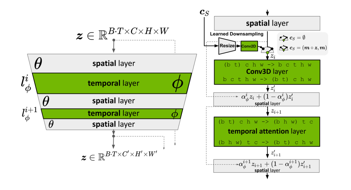
LDM architecture in NVIDIA’s “Align your Latents: High-Resolution Video Synthesis with Latent Diffusion Models”.****

the spatial layers are shown in gray and are parameterized by theta. note that theta remains unchanged because we are basically freezing the weights of the image LDM backbone. this means we are only training for the temporal layers in green, which are parameterized by phi.

this is handy because we can already get a spatially-aware image, but now the challenge is extending this to videos, or the time dimension. a temporal layer is either a temporal convolution layer, or a temporal attention layer.

the convolution layers had a similar approach to Make-a-video by sliding a 1D convolution along the time axis, but in latent space. this captures local temporal smoothness by capturing motion from frame t to frame t+1.

the attention layers work similar to that of LLMs, but instead of words being attended to, it is a stack of frames over time. this is how we ensure global coherence, in a similar way we know the “He” in a paragraph refers to “Sammy” who was introduced in the very first sentence.

while NVIDIA solved a big part of the compute bottleneck with latent diffusion, not much work up to this point commented on the training data. in November 25, 2023, Stability AI emphasized dataset quality and scale and its influence on the results [5].

Stability AI employed multiple strategies like clip annotation using an image captioner, or filtering based on motion, excessive text, and aesthetic value, they created Large Video Dataset (LVD) which contained 580M annotated video clip pairs, which amounted to roughly 212 years of content. they demonstrated the value of scaling high quality data pipelines rather than architectural novelty.

current models

today, the ai video generation scene has exploded with many different models to the point i can no longer keep track of all of them. that is to say they can be broadly categorized into closed source and open source models.

some of the leading open source models include Wan2.1 (Alibaba), Stable Video Diffusion (Stability AI), and HunyuanVideo (Tencent). for the sake of brevity of an already long article, i will just focus on Wan2.1 [6].

Wan is essentially a synthesis of a lot of the core technology that has been employed over the past 5 or so years. it integrates many of the major breakthroughs at a very large scale including LDMs, diffusion transformers (DiTs) [7], space-time modelling from models like Lumiere [8], and of course highly curated datasets.

the first thing they did was curate a high quality dataset. they prioritized high quality, high diversity, and substantial scale. the dataset comprised billions of videos and images. they used a large number of filtering techniques including (and not limited to) text detection, aesthetic evaluation, NSFW scoring, watermark and logo detection, black border detection, overexposure detection, synthetic image detection, blur detection, and clips greater than 4 seconds long.

Wan is based on the DiT architecture which is comprised of the Wan-VAE, the diffusion transformer, and a text encoder.

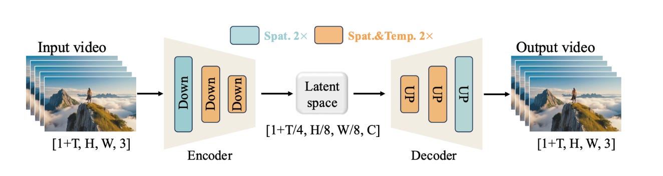
visual representation of the Wan-VAE.

Wan created a custom VAE, called the Wan-VAE. VAEs play an important role in learning latent representations from high dimensional data like videos. designing VAEs are usually difficult for videos because we need to capture both spatial and temporal dimensions. the high dimensionality of videos increases memory and compute costs, making it hard to scale to long videos.

the Wan-VAE includes several optimizations such as replacing GroupNorm layers with RMSNorm layers to help preserve temporal causality. they also implemented a feature cache mechanism to improve inference efficiency.

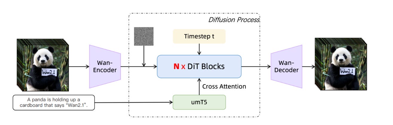
overview of the Wan2.1 diffusion transformer pipeline.

Wan extends the DiT from a spatial image transformer into a spatio-temporal multimodal video transformer by patchifying in 3D and using cross-attention to inject text input and time conditioning into every block.

the text encoder also uses umT5 to encode input text which was found to have strong multilingual capabilities (chinese and english) and has faster convergence.

another important note about Wan is its usage of flow matching during pretraining. recall in classic diffusion, we are training a model to try and predict the “noise” delta at each step so that at inference we can start from noise and reverse the process iteratively.

flow matching works by using ordinary differential equations to directly interpolate between pure noise and the real data without the usage of discrete noisy steps [9]. without getting into the math, flow matching reveals that we can predict a more stable signal instead of predicting added noise which is inherently random. as a result, generated videos exhibit smoother temporal consistency compared to traditional noise-prediction diffusion.

as an open-source model, Wan has offered rare transparency into how state-of-the-art video diffusion works, giving us clues about the otherwise opaque design choices behind closed-source systems like Sora and Veo.

closing

these models show how far video generation has come in just a few years. as models edge closer to generating fully photorealistic, long-form videos on demand, i ask myself: what happens when anyone can create their own movie as easily as writing a paragraph of text?

---

notes

1. https://arxiv.org/abs/2204.03458
2. https://arxiv.org/abs/2210.02303
3. https://makeavideo.studio/Make-A-Video.pdf
4. https://arxiv.org/abs/2304.08818
5. https://arxiv.org/abs/2311.15127
6. https://arxiv.org/abs/2503.20314
7. https://arxiv.org/abs/2212.09748
8. https://arxiv.org/abs/2401.12945
9. https://arxiv.org/abs/2210.02747